4 Statistical methods

There are two cardinal rules when analyzing complex survey data:

always use a strata and a weight variable; and
when analyzing subgroups, always use a subpopulation statement instead of excluding observations from the dataset.

Rule #1: In many observational studies, we assume that the cohort that we have is a simple random sample from the target population of interest. Sometimes that assumption is not correct, but we have no way to know it so we make it anyway. However, in ARIC community surveillance we intentionally sampled in such a way that the observations we have in the dataset are an intentionally biased representation of the actual hospitalizations that happened in the communities. The benefit for this bias was better representation of subgroups of interest and lower overall standard errors for our final estimates.² Therefore, when analyzing ARIC community surveillance data, we have to use statistical procedures and software that account for this sampling strategy in order to make statements about the ARIC communities. If we do not use these special methods, then we cannot make inference about any really meaningful population quantity of interest (e.g., rates of MI).

Rules #2: We often want to calculate summary statistics in particular subgroups (e.g., men vs. women). The standard way to approach this problem is to restrict the dataset to observations of men, then calculate the summary statistic, and repeat for women. However, using this approach with survey data ignores the sampling design in a meaningul way. Let us assume there are some strata with extremely small counts, and one has only 3 observations, all of which are women. An analysis that excluded all women would implicitly eliminate this particular stratum from the sampling design, even though there might have actually been men in that stratum in the population (we just did not get any in our particular sample). Not using all of the strata will bias the standard errors for our estimates as well. Therefore, complex survey software always has an option for how to specify analyses in a subpopulation. You should always use these options.

Here is a table of the potential survey sampling variables and when you would use them:

Outcome	Years	Age group	Stratum variable	Weight variable
CHD/MI	1987-2014	35-74	`NESTVAR2`	`SAMWT_TRIM`
CHD/MI	2005 - 2014	35-74	`NESTVAR2`	`SAMWT_TRIM`
CHD/MI	2005 - 2014	35-84	`NESTVAR_COMBN`	`SAMWT_TRIM`
CHD/MI	2005 - 2014	75-84	`NESTVAR_OLD`	`SAMWT_TRIM`
HF	2005 - 2014	55+	`SAMSTRAT2`	`SAMWTHF`

Finally, we always analyze a subpopulation of the full data that excludes certain observations from the Washington County site for particular years, either because of low counts or because there were administrative issues with using the data for analyses. Therefore, for all community surveillance analyses, you should subset to the observations where the following condition is not met: the site is Washington County, and the year is before 1995 or equal to 2003 or 2004. See below for a code implementation of this population subsetting.

4.1 Exploratory data analysis

Standard summaries, such as means, variances, counts, proportions, and quantiles are all available in survey methods packages. Please explore the functions in the survey package in R to find the function you need.

Some examples in R:

library(survey)
d <- svydesign(ids = ~EVENT_ID, strata = ~NESTVAR2, weights = ~SAMWT_TRIM, data = subset(s14_analysis, !(CENTER == "W" & (YEAR < 1995 | YEAR == 2003 | YEAR == 2004))))  # Set up the survey object. This is basically a data frame with some extra information about the sampling design so that you don't have to repeat this information about strata and weights in future steps.

svymean(~DDAYS, d)

##         mean    SE
## DDAYS 41.357 0.934

svymean(~RACE, d)  # proportions of each race

##          mean     SE
## RACEB 0.29034 0.0013
## RACEW 0.70966 0.0013

svytotal(~RACE, d)  # totals for each race

##        total     SE
## RACEB  91936 424.45
## RACEW 224717 475.64

svytable(~ MIDX3 + YEAR, d) %>%  # total number of hospitalizations in each category of MIDX3 over time
  as_tibble() %>%
  ggplot(aes(x = as.numeric(YEAR), y = n)) + 
  geom_path(aes(group = 1)) + 
  facet_wrap(~ MIDX3) +
  xlab("Year")

4.2 Modeling outcomes that are not population rates

When we are not trying to estimate a population rate, things remain fairly simple. We just use the survey version of the linear model we are trying to fit, such as a logistic regression model. For example, let’s say we wanted to know what the odds of being black vs. white were among the different types of MI, adjusted for year and sex. That would be

f <- svyglm(factor(RACE) ~ MIDX3 + YEAR + GENDER, family = quasibinomial(), d)

broom::tidy(f) %>%
  filter(str_detect(term, "MIDX3")) %>%  # choose only the terms you're interested in
  mutate(odds_ratio = exp(estimate)) %>%  # exponentiate the parameter estimates to get the ORs
  select(term, odds_ratio)

## # A tibble: 5 x 2
##   term         odds_ratio
##   <chr>             <dbl>
## 1 MIDX3NO-HOSP      0.650
## 2 MIDX3NO-MI        1.07 
## 3 MIDX3PROBMI       0.905
## 4 MIDX3SUSPMI       0.732
## 5 MIDX3UNCLASS      0.827

4.3 Modeling population rates

Now we come to the hard part. But actually, we’ve already done the hardest part of the work when setting up the data!

To find event rates in the ARIC population, we use log linear models (i.e., regression models with a log link function and a Poisson error distribution). Since we’ve already calculated the appropriate offset for each observation previously, we can just fit the model and use the predicted mean values to get the rates in the ARIC population. Of course, that will be the rate per person, and we usually report rates per 10,000 persons in ARIC.

f <- svyglm(MI3 ~ as.numeric(YEAR) + RACE + AGEGRP + GENDER, offset = log(offset), family = quasipoisson(), d)

prediction_dataset <- modelr::data_grid(s14_analysis, YEAR, RACE, AGEGRP, GENDER)  # Need to specify the values of the predictors that you want the means for. In this example, we are looking at the trend in MI across all race, sex, and age groups.

preds <- modelr::add_predictions(prediction_dataset, f) %>%
  mutate(rate = exp(pred) * 1000)

preds %>%
  ggplot(aes(x = as.numeric(YEAR), y = rate, color = AGEGRP)) +
  geom_path(aes(group = AGEGRP)) +
  facet_grid(RACE ~ GENDER) +
  xlab("Year") +
  scale_color_brewer()  # Default ggplot2 color palette is not color-blind friendly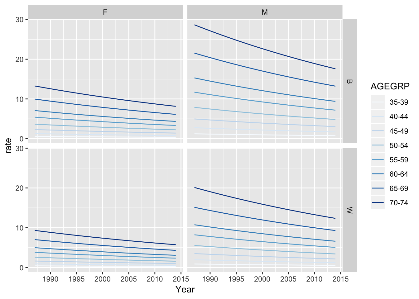

4.3.1 Age standardization (optional)

Some investigators, after adjusting for age, like to standardize the predicted rates to a particular population with a particular distribution of ages. In ARIC analyses, the CSCC has traditionally standardized to the age distribution in the 2000 Census. The proportion of the US population in each age group we typically use is:

AGEGRP	USPOP2000	proportion
35-39	22706664	0.0552667
40-44	22441863	0.0559188
45-49	20092404	0.0624575
50-54	17585548	0.0713610
55-59	13469237	0.0931695
60-64	10805447	0.1161379
65-69	9533545	0.1316322
70-74	8857441	0.1416799

Using these proportions, you can obtain a weighted average of the rates across the age groups to produce an age-standardized rate.

Sampling within homogeneous strata produces lower variance parameter estimates later on. This result is fundamental to sampling theory.↩